ECE4960_FastRobots

layout: page title: “Lab 3” permalink: /ECE4960_FastRobots/lab3/

Back to home

Lab 3: TOF and IMU

Lab 3a Time of Flight Sensors

1. The TOF I2C address is 0x29, which is the expected address based on the new set of sensors acquired for this class.

2. setDistanceModeShort() is suitable for applications in environments with lots of noise. In addition, the sensor needs a shorter time to report a measurement. However, this mode is limited to 1.3 meters. An example application of this mode is a TOF sensor placed at the front of the robot for object avoidance.
   setDistanceModeLong() is suitable detecting objects up to maximum distance (4 meters) applications, but is vulnerable to ambient noise and takes longer to measure. An example application of this mode would be for mapping the environment. setDistanceModeMedium() averages the benefits and drawbacks of the short and long modes. This mode would be suitable for a sensor that is doing mid-range sensing or mix range sensing.

3. I collected 100 readings at variosu distances and surfaces textures to compare accuracy (measured by error), repeatability (measured by standard deviation), and ranging times. Note that I collected timestamps and calculated the durations in post-processing to prevent slowing down my code.

void loop()
{
  // setup delay for movin sensor
  if(readCount < 100)
  {
    readCount++;
  }
  else
  {
    Serial.println("100 reads, pausing for 10s to move sensor");
    readCount = 0;
    delay(10000);
  }
  
  // READ DIST FROM TOF1
  
  float time0 = millis();
  tof1.startRanging(); //Write configuration bytes to initiate measurement

  while (!tof1.checkForDataReady())
  {
    delay(1);
  }

  int distance1 = tof1.getDistance(); //Get the result of the measurement from the sensor
  tof1.clearInterrupt();
  float time1 = millis();
  tof1.stopRanging();
  float time2 = millis();

  Serial.print(distance1);
  Serial.print(", ");
  Serial.print(time0);
  Serial.print(", ");
  Serial.print(time1);
  Serial.print(", ");
  Serial.print(time2);

  Serial.println();
}

Color, texture, distance (mm)	Avg error	Standard deviation (mm)	Ranging time (ms)	Stop ranging time (ms)
Black, fabric, 127	4.9%	1.55	52.9	52.9
White, paper, 127	0.0036%	1.11	52.1	52.1
Black, fabric, 254	3.12%	1.08	52.1	52.1
White, paper, 254	0.24%	1.07	52.3	52.3
White, wall, 900	5.68%	1.71	53.0	53.0

In short distance mode, we can see how distance and surface color/texture affects the TOF sensor readings. We see that the dark, fabric surface leads to higher error. This makes sense as the rough surface texture probably deflects the waves at a larger deviation from incidence angle. We also see that the ranging time is larger for longer distances, which makes sense as the time of flight over larger distances must be longer. For all readings, we see that the estop ranging time is the same (to millimeter resolution). This is also expected as it takes almost no time to execute a stop command.

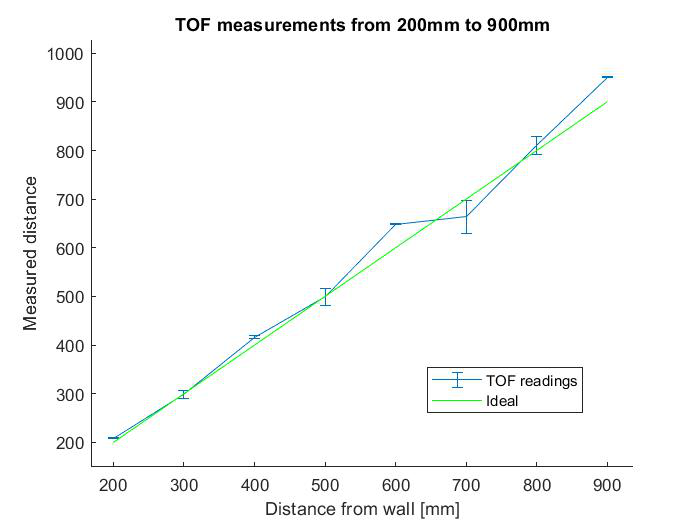
I also plotted sensor readings from 200mm to 900mm. We see that short distance mode does decently well up until 600mm, then the readings become less accurate and less repeatable.

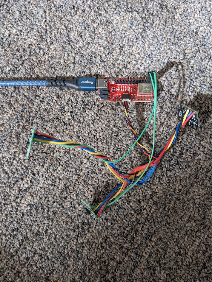
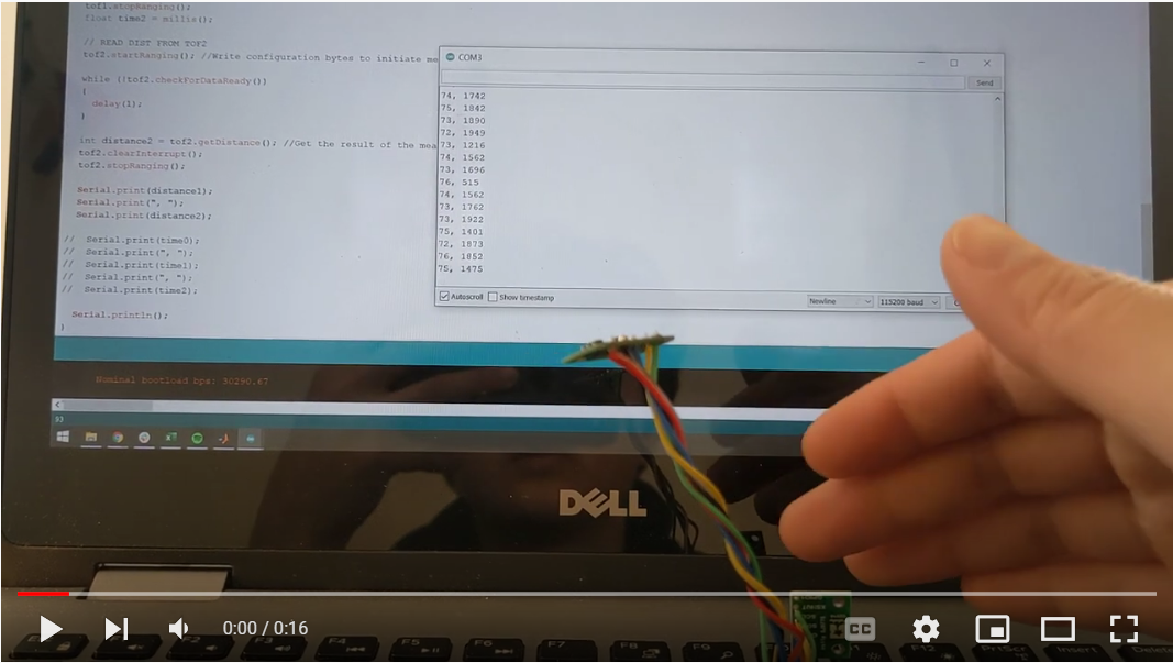
1. Using the XSHUT pins on the TOF sensors, I was able to set the sensors to different addresses and collect readings from both simultaneously.

void setup()
{
  //  set outputs, set TOF 2 XSHUT to low
  pinMode(XSHUT_pin1, OUTPUT);
  pinMode(XSHUT_pin2, OUTPUT);
  digitalWrite(XSHUT_pin1,HIGH);
  digitalWrite(XSHUT_pin2,LOW);

  Serial.begin(115200);
  Wire.begin();

  tof1.setI2CAddress(tof1_address); //change address of sensor before powering up next one
  
  if (tof1.begin() != 0) //Begin returns 0 on a good init
  {
    Serial.println(" TOF 1 failed to begin. Please check wiring. Freezing...");
    while (1)
      ;
  }

  digitalWrite(XSHUT_pin2,HIGH); // set TOF 2 XSHUT to high after TOF 1 address set

  if (tof2.begin() != 0) //Begin returns 0 on a good init
  {
    Serial.println("TOF 2 failed to begin. Please check wiring. Freezing...");
    while (1)
      ;
  }

  tof1.setDistanceModeShort();
  tof2.setDistanceModeShort();
}

void loop()
{  
  // READ DIST FROM TOF1
  
  tof1.startRanging();

  while (!tof1.checkForDataReady())
  {
    delay(1);
  }

  int distance1 = tof1.getDistance();
  tof1.clearInterrupt();
  float time1 = millis();
  tof1.stopRanging();
  
   // READ DIST FROM TOF2
  tof2.startRanging();

  while (!tof2.checkForDataReady())
  {
    delay(1);
  }

  int distance2 = tof2.getDistance();
  tof2.clearInterrupt();
  tof2.stopRanging();

  Serial.print(distance1);
  Serial.print(", ");
  Serial.print(distance2);

  Serial.println();
}

Lab 3(b) IMU

Setup the IMU

1. The IMU I2C address is 0x68. When converted from hexadecimal to binary, this address matches the address b1101000 (listed in binary) in the ICM-20948 datasheet for when the AD0 pin is set to low. At first, the sensor failed to initialize because I top the AD0 pin on high in the code.

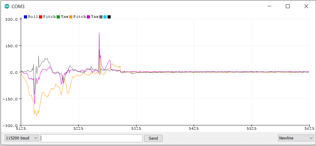
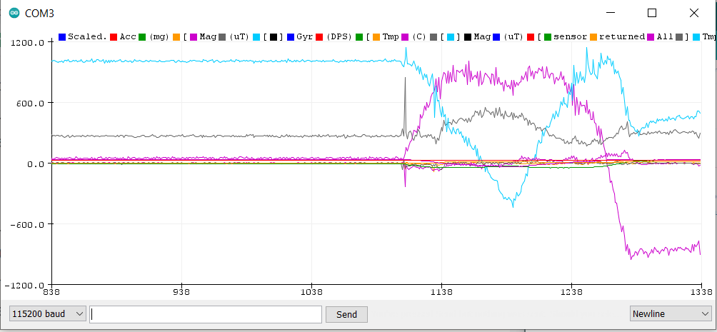
This issue was resolved promptly after I set AD0 to low: #define AD0_VAL 0 As I flipped the IMU in my hand, the Serial Plotter shows gyroscope angles in blue, magenta, and brown lines. I tried to keep the board rotating about itself, but inevitably moved it a bit. This is reflected in the mostly flat lines clumped toward the middle with some fluctuations. We see a little bit of noise in the readings, but not a whole lot. This indicates that the hardware LPF is probably activated. We will verify that in the next section

Accelerometer

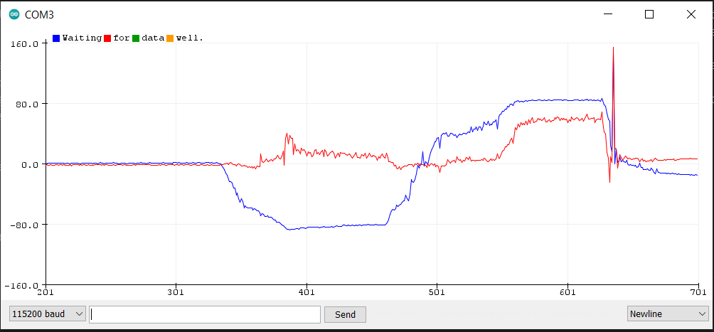
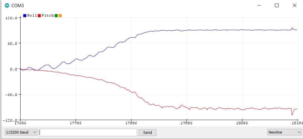
1. The roll (top) and pitch (bottom) angles from the accelerometer are accurate within a few degrees. The signal is not too noisy at all, let’s see if we can improve it with a low pass filter.

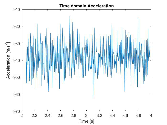
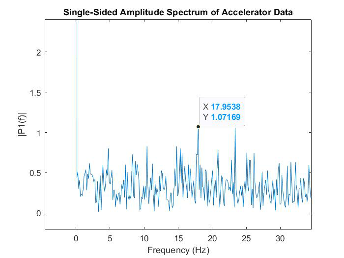
1. By performing FFT on the time-domain signal (top) from tapping the sensor, we can see throuhgh the frequency response (bottom) that there really is some high frequency signal.

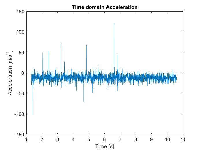
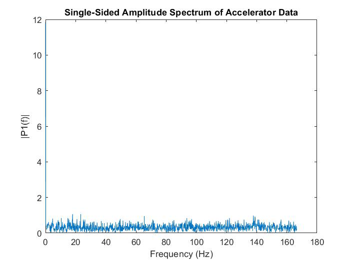
To verify the high frequency response is actually noise and should be to cut out, we will plot the response of the accelerometer sitting still.

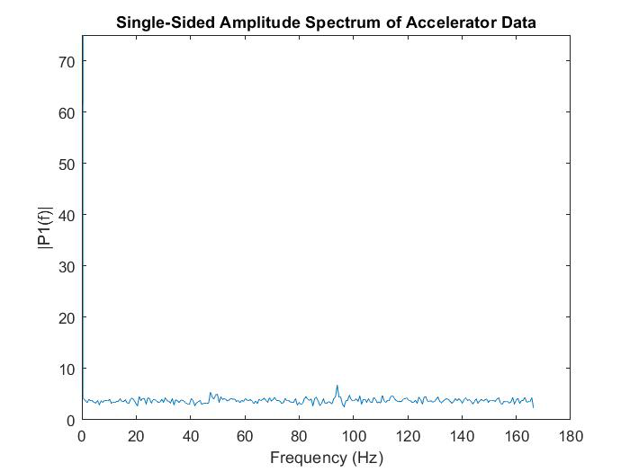
We see that there is almost no noise besides the peak near 0Hz (that is just the DC signal), so all of the high frequency response that we saw previously actually resulted from the accelerometer moving. This is not too surprising, as we know that the sensor itself has a LPF that can be activated. We can choose a local maximum of f_c = 18Hz, which gives ALPHA = 0.31.

  // pull sensor values
  float a_x = sensor->accX();
  float a_y = sensor->accY();
  float a_z = sensor->accZ();

  // calculate roll, pitch angles in degrees 
  float temp_roll = atan2(a_y, a_z) * RAD2DEG;
  float temp_pitch = atan2(a_x, a_z) * RAD2DEG;

  // LPF
  roll_a = ALPHA * temp_roll + (1 - ALPHA) * roll_a;
  pitch_a = ALPHA * temp_pitch + (1 - ALPHA) * pitch_a;

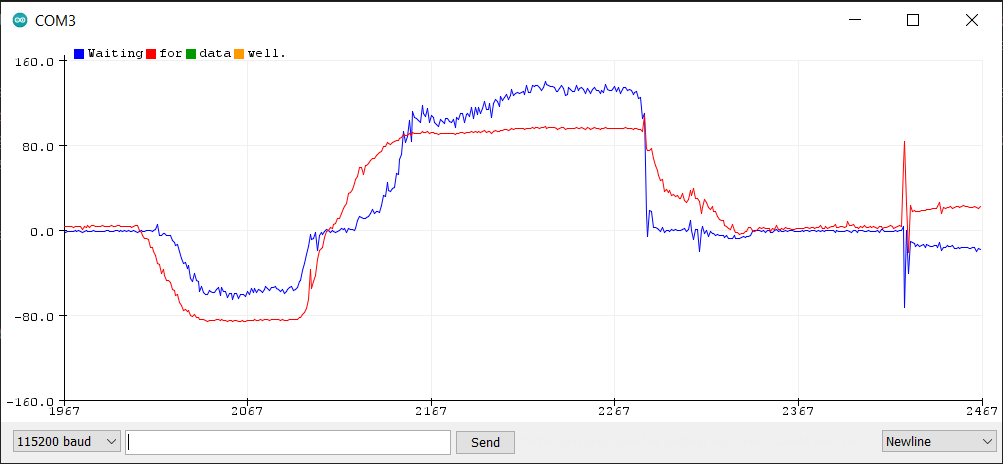
After applying the self-implemented LPF, the response is about the same as before

Gyroscope

1. By multiplying the gyroscope data with time lapse since the last sensor read, I can calculate the angle of the IMU.

//  determine time elapsed since last gyro read
float d_time = 0.001 * millis() - timestamp;

// pull gyro values 
float d_roll = sensor->gyrX();
float d_pitch = sensor->gyrY();
float d_yaw = sensor->gyrZ();

roll_g = roll_g + d_roll*d_time;
pitch_g = pitch_g + d_pitch*d_time;
yaw_g = yaw_g - d_yaw*d_time;

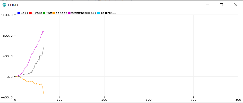
The gyroscope data is much less noisy. However, the values drift away rapidly.

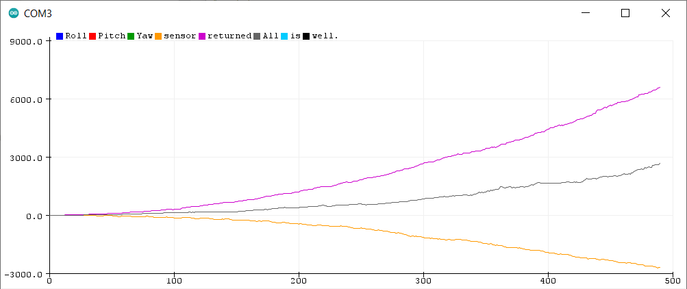
The drift only gets worse as we decrease the sampling frequency. As the error dominates the relatively non-changing angle accumulates at each time step gets larger.

1. Using the accelerometer data in a complimentary filter, I am able to get more stable roll and pitch readings.

// pull accelerometer values
  float a_x = sensor->accX();
  float a_y = sensor->accY();
  float a_z = sensor->accZ();

  // calculate roll, pitch angles in degrees from accelerometer
  roll_a = atan2(a_y, a_z) * RAD2DEG;
  pitch_a = atan2(a_x, a_z) * RAD2DEG;
  
  //  determine time elapsed since last gyro read
  float d_time = 0.001 * millis() - timestamp;
  
  // pull gyro values 
  float d_roll = sensor->gyrX();
  float d_pitch = sensor->gyrY();
  float d_yaw = sensor->gyrZ();

  roll_g = (roll_g + d_roll*d_time) * (1 - ALPHA) + roll_a * ALPHA;
  pitch_g = (pitch_g + d_pitch*d_time) * (1 - ALPHA) + pitch_a * ALPHA;
  yaw_g = yaw_g - d_yaw*d_time;